Predator - prey interactions
Introduction
In the Lotka-Voterra common resource competition exercise, we saw that the dynamics of any given species can be influenced by those of other species which are competing with it for resources. This often takes place within a particular trophic level. Two species of ungulates could feed on grasslands within a common area, for instance. In nature, population dynamics are also regulated by species across trophic levels – the dynamics of predator populations are influenced by how many prey individuals are in the community is a common example of this. These predator-prey interactions are also described by Lotka-Voterra equations. In this case these are a pair of differential equations describing the population dynamics of one species at one trophic level as a function of the dynamics of species within another other trophic level. Although it is most commonly discussed in a “predator-prey” context, the framework here can me modified to suit other scenarios such as plant-herbivore, parasites-host interactions.
Exponentially growing prey
Due to the greater complexity of the relationships involved when modelling two species interactions we will not be using derrived equations. Rather we will use the differential equation as our model. We will be using the deSolve package to help us solve these differential equations which we will then plot as normal.
The simplest Lotka-Volterra predator-prey equation considers a prey or victim species \(V\) that grows exponentially at a rate \(r\), and shrinks as it gets consumed by predators \(P\), which attack the prey they encounter at a fixed, per-capita (i.e. dependent on the number of predators and prey) rate \(\alpha\):
\[\frac{dV}{dt} = rV - \alpha VP\]
The population of the predators \(P\) grows as it converts the prey which it encountered and consumed into new predator individuals at a fixed per-captia rate \(\beta\), and shrinks due to a constant per-capita mortality rate \(d\):
\[\frac{dP}{dt} = \beta \alpha VP - dP\]
Let’s take a look at what this model implies. When there are no predators in the community (i.e. \(P = 0\)), the prey species \(V\) grows due to simple exponential growth (\(rV\)). If there were limiting resources then the prey would grow until its carrying capacity but we will ignore that aspect in this example for simplicity. Conversely, when there are no prey individuals in the community (i.e. \(V = 0\)), the predator popultion has no way to sustain its growth grow and exponentially declines towards zero \(-dP\).
The rate of growth of the predator population increases when prey are abundant and predators are few. On the other hand, when there are plenty of predators, the prey population suffers and cannot grow very quickly. We can get some suggestion that this predator-prey relationship might lead to some sort of population cycling – as the prey population grows, so too does the predator popuplation, which in turn reduced the number of prey which in turn reduces the number of predators allowing the prey to increase once more.
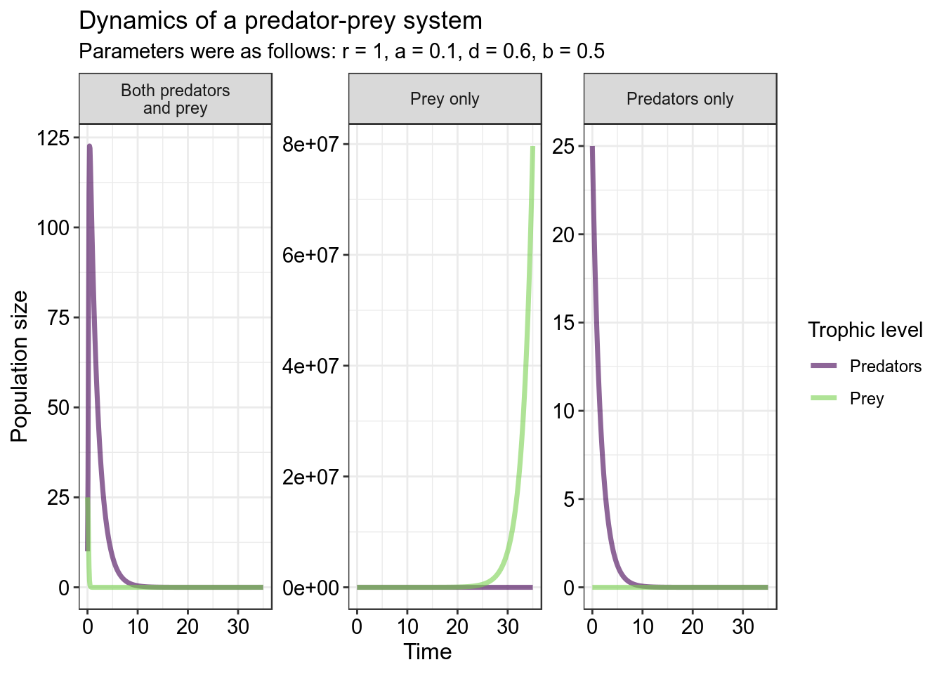
As expected, cyclic population dynamics are common in predator-prey systems:

In the first plot above, the system begins with 25 prey and 10 predators – cyclic dynamics shortly ensue. In the middle panel, there are no predators in the beginning, so the prey population simply grows exponentially. In the third panel, there are no prey individuals in the system – so, the predator population shrinks exponentially to zero.
Logistically growing prey
In the previous model, prey experience exponential growth when predators are absent – in other words, the predators are the only factor regulating the prey population’s dynamics. Of course, this doesn’t generally happen in nature. Even when predators are absent a prey population will eventually level off at some carrying capacity dictated by the available resources within the habitat.
To incorporate this aspect into our equations we can modify the above prey equation by incorporating density-dependent growth simply by adding a term to represent the population’s carrying capacity:
\[\frac{dV}{dt} = rV - \alpha VP - cV^2\]
Where the value of the carrying capacity can be calculated as \(K = \frac{r}{c}\) which has been taken from logistic population growth. So if you want a very large \(K\) then make \(c\) very small. We keep the predator population dynamics the same as before:
\[\frac{dP}{dt} = baNP - dP\]
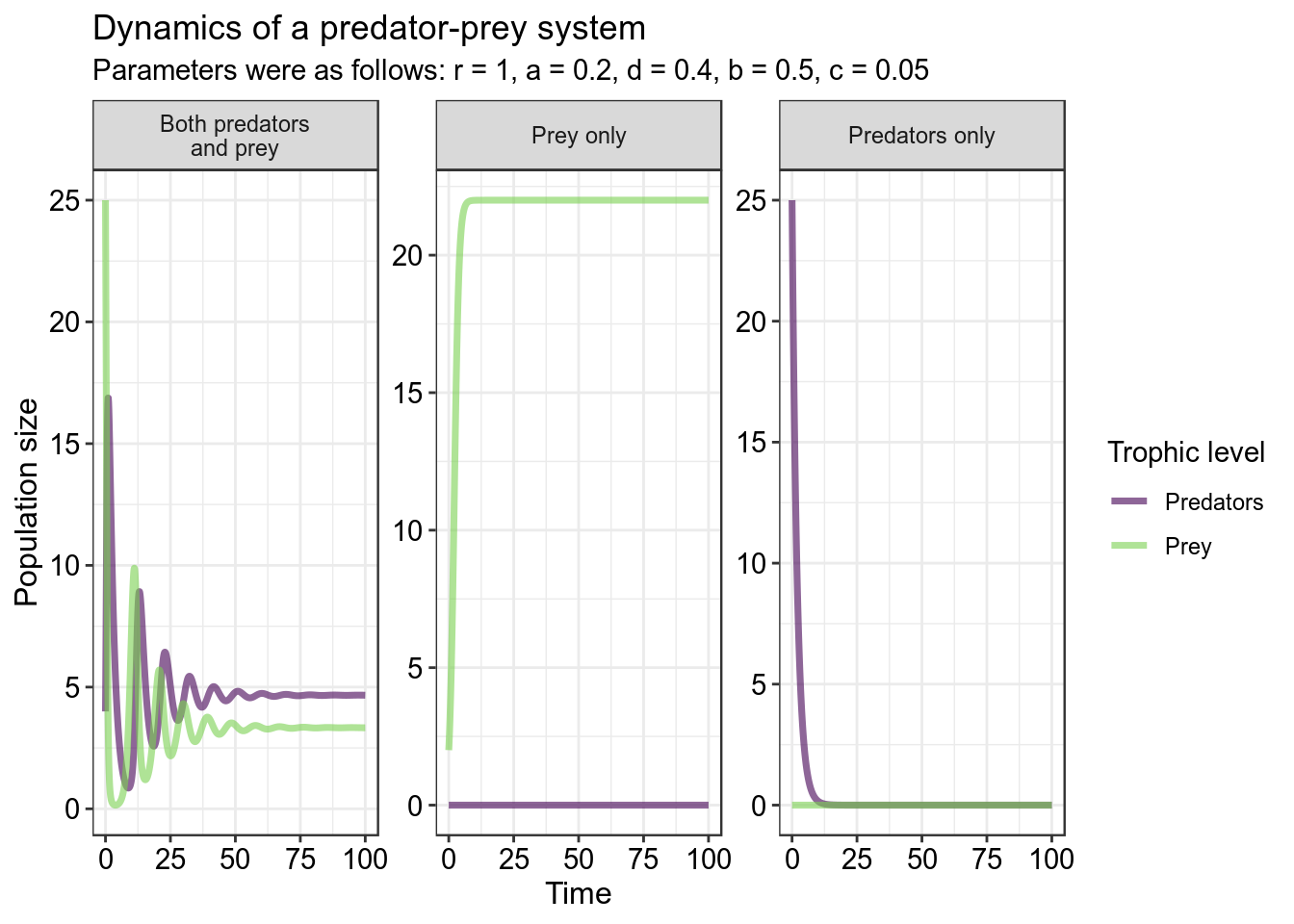
With these new equations, when predators are absent from the community, the prey species grows exponentially but it is then restricted by its own abundance in a similar manner to how the logistic growth equation would function. One possible outcome in this case is stabilised population cycles - in other words, the predator and prey populations can cycle up and down until they reach a joint equilibrium:

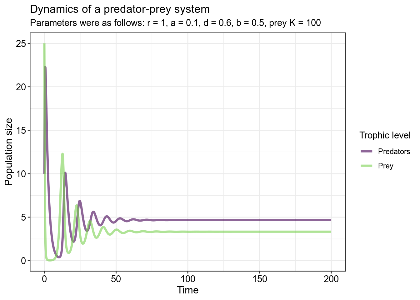
Note that in the middle graph, the prey population grows logistically to its carrying capacity of 10 when no predators are present. If we run this system out longer, we see that the populations eventually stop cycling as they reach an equilibrium when both predator and prey are present in the system:

Parameter exploration
Download Lotka-Voltera predator prey app here and answer the questions on the prac worksheet.
This app requires several parameters and the user interface is quite cluttered. The default app viewer which you have likely been using for the previous apps will not work well and it will be better for you to run the app in your web browser. To do this run the app file from RStudio and then click Open in browser. Once open in your web browser do not close the app file as this will crash the browser page. To see all the app options in the browser app you will need to zoom out to approximately 80%.
Worksheet questions
Question 1
An important starting point for any model is understanding what the different aspects of the equation represent. One can access this information from the units that a particular parameter is measured or reported in. Give the units of:
- \(\alpha\) (3)
- \(\beta\) (3)
Question 2
Briefly explain how the term \(cV^2\) produces similar outcomes to the term \(\left(1-\frac{N}{K}\right)\) which we have used in the exponential and logistic growth practical (3)
Why do we only incorporate carrying capacity (in the form \(\left(\frac{r}{c}\right)\) in today’s example) into the prey population growth equation but not into the predator population growth equation (2)
Question 3
Which model parameters influence the magnitude and frequency/periodicity of the fluctuations of the predator and prey populations when there is no carrying capacity (4)
Question 4
Both the incorporation and exclusion of carrying capacity results in the populations reaching some kind of equilibrium. This equilibrium can be stable or unstable. Describe how the parameters of the predator and prey populations interact with each other as the populations approach this equilibrium and state the kind of equilibrium reached
- without a prey carrying capacity (4)
- with a prey carrying capacity (4)
Make specific reference to the ZNGI curves.
Question 5
Under what conditions will the predators not be able to successfully establish themselves and thus become extinct from the community (4)
Question 6
Discuss the application of the second figure – what information does it convey and what could it be used for in a conservation/management scenario (3)