Habitat selection

Introduction

During our previous practicals we have been modelling population growth through time and under different levels of resources. These two parameters are both very important but they are lacking in their ability to fully represent the world we (and the animals and plants we are interested in modelling) live in. To provide a better picture we can incorporate a more spatial aspect into our calculations. This doesn’t necessarily need to be in the form of actual distances and coordinates but rather presenting our population of interest with a “choice” between two or more habitats which differ in resources and abiotic characteristics.

It’s not just wild animals that make these decisions, humans do this too. We choose between places we would like to live, for instance, and decide on this particular place based on the resources available to us and the costs and benefits of living in this area. Although we all might like to live in a nice house in the best area we aren’t all able to do so. Nice houses are generally more expencive and so you’ll have larger loan repayments. They are also bigger and require more energy and so your rates and maintenence costs will likely be higher. Houses in nice areas are also generally further away from work places and so you’ll need to travel further which adds to the expences. Contast this with, say university residence accommodation. Here the houses aren’t houses at all but rather flats or apartments and so the living area is smaller and, therefore, the rates and resources required to maintain these “houses” are much lower. These areas are also generally right next to or very close to your “work” places and so the energy (or travel costs) are substantially lower. Thus, humans incorporate these factors and any potential resource limitations when we decide where we would like to live.

Similarly, in natural settings animals are presented with a host of factors that need consideration when deciding on which habitats to live in. These could be, for instance, climate, food types, competitor presence, and predator presence. As you have likely realised by now, it is quite difficult to model all of these parameters in one equation although it is possible.

To help us better understand and predict how animals will select between habitats ecologists have developed several important models. Today we will look at two of these, the Ideal-Free Habitat Selection model and the Ideal-Despotic Habitat Selection model.

Ideal-Free Habitat Selection

Under this model each habitat has a set basic or intrinsic level of habitat suitability for a given potential inhabitor, however, as we have already discussed, not all habitats are equally suitable. Dolphins have a higher preference for open oceans than they do for tidal pools, and they have absolutely no preference for savanna plains. Elephants, on the other hand, prefer savannas to tundra or snowy alpine regions (just ask Hannibal how trying to march elephants over the Alps went for him!).

But it’s not just the intrinsic requirements of an animal that dictates which habitat to live in. If there is high competition in a particularly good habitat, an animal may be better off in a habitat with intrinsicly lower resources but less competition. This kind of scenario is (in part) described by the ideal-free habitat selection model - that animals will distribute themselves between different habitats in ratios proportional to the amount of resources available to them. Thus, habitats or patches with higher intrinsic resource levels will support a greater number of individuals. The result of this Ideal Free examlpe is that resource competition between individuals consuming the same resources will be minimised and the energy uptake of the individuals will be maximised.

The “ideal” part of this model’s name refers to the assumption that the animals are awear of the resources available to the animals across all the patches whilst the “free” component reminds us of the assumption that the animals are free to move between patches at no cost to themselves.

The model is designed to predict habitat suitability across habitats in which foragers will have equal resource gains and rates of resource uptakes such that at an equilibrial state each individual will not be able to improve on it’s resource availability by moving to a new patch. We can use the following equation to describe this kind of habitat suitability:

\[S_i = B_i - f_i(d_i)\]

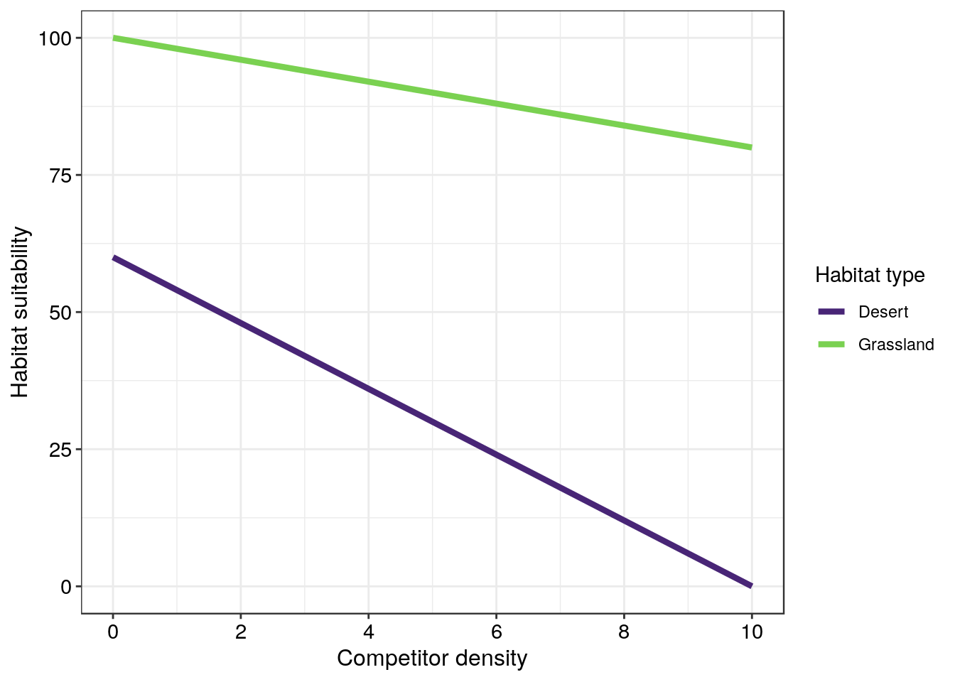
Here \(S_i\) is the realised habitat suitability after subtracting the effect (\(f_i\)) that fellow competitors have on the intrinsic habitat suitability (\(B_i\)) multiplied by the number of competitors \(d_i\) present in the habitat. In the example figure below there are two habitats - a desert and a grassland. These two habitats differ in both their intrinsic suitability and their response to increased inhabitant presence. The figure suggests that grasslands are generally more suitable places to live than deserts and that the impact that new individuals have on the habitat suitability declines more quickly in deserts than in grasslands.

Ideal-Despotic Habitat Selection

Although there are examples of the above model being successfully applied to natural (and artifical) scenarios, it can be modified when some of its many assumptions fail to be met - a common one being the “free” movement assumption. Free movement between patches can be restricted when potential colonisable patches are already controlled by despots/dictators. From a human perspective once someone comes to own a piece of property it becomes quite difficult to remove that person and take ownership of the area. We can describe this phenomenon verbally as the lowering of a patch’s suitability for future colonists due to the presence of current resident individuals which can be expressed mathematically as:

\[T_i = S_i (1-t(d_i))\]

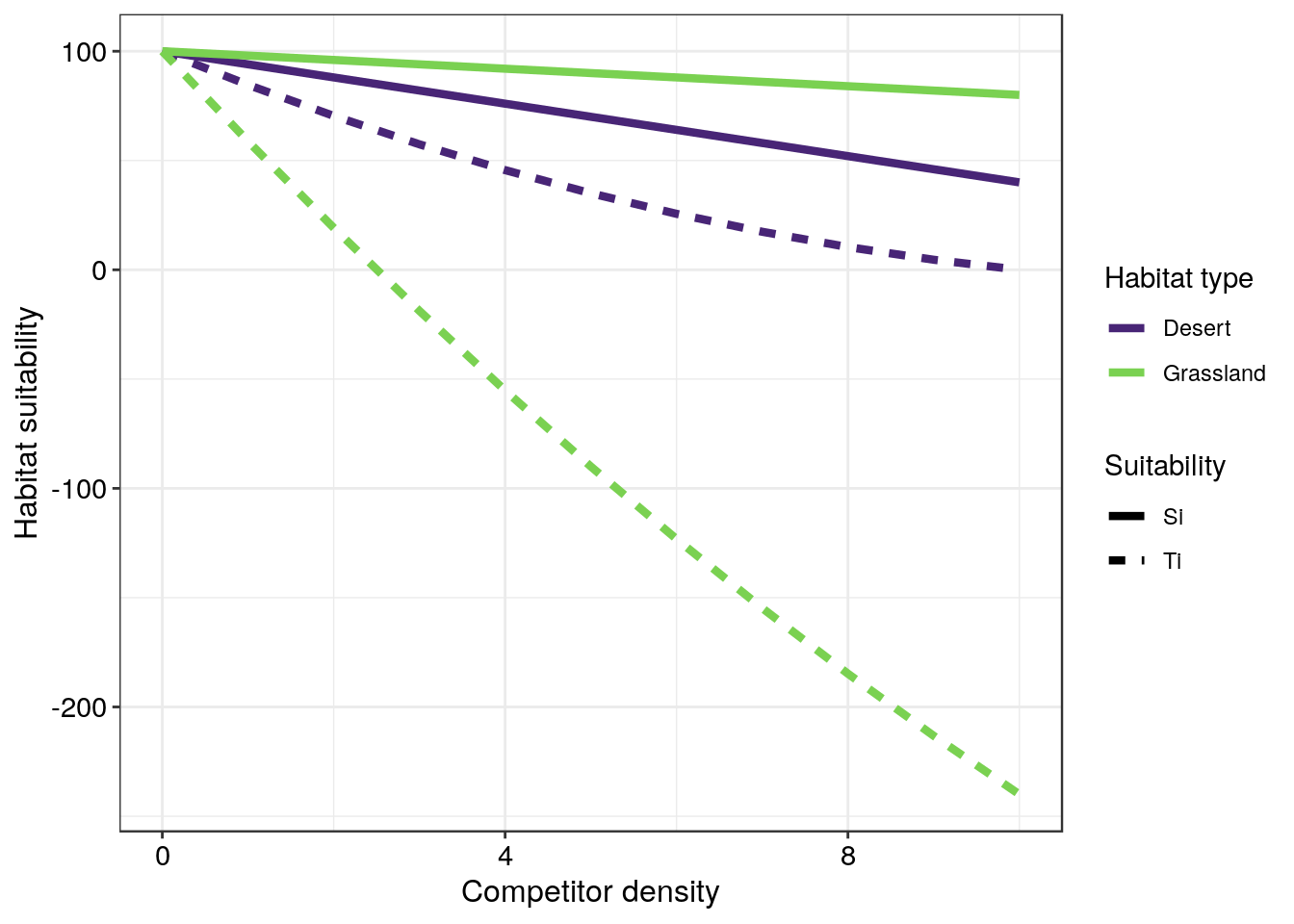
where \(T_i\) is the apparant suitability of habitat \(i\) for an unsettled or habitat searching individual, \(S_i\) is the realised, or actual suitability of habitat \(i\) (taken from the IFHS model defined above) together with a reduction in suitability attributed to the resistance (\(t\)) of the current occupants (\(d\)) of the \(i^{th}\) habitat. \(t\) can technically take any real value but for now we will restrict it to between 0 and 0.2. The figure below depicts the difference between the realised or actual suitability (solid lines) and the apparant suitability (dotted lines).

Simulating settlement

At the beginning of this exercise it was mentioned that our previous practicals failed to specifically address the spatial aspect of population dynamics. The two models presented in this practical have attempted to do that but in doing so we have excluded the temporal component. Thus, our model outputs are static snapshots of habitat suitability at varying competitor densities which could be at the beginning of a colonisation event or nearing the end. In real scenarios we might rather be interested in simulating the entire colonisation process from beginning to end to model habitat selection of say two habitats by colonisers where initially both habitats are bare.

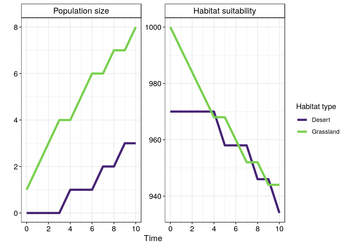
The underlying principle here is to use if statements to compare the suitability of two habitats at each point in time and add individuals to the more suitable habitat whilst adjusting the habitat suitability based on the presence of new inhabitants. An if statement is a logical operator that compares one variable to another or to a fixed value. The result of this comparrison could return either a TRUE or a FALSE response. After conducting the comparison the if statement will then carry out one of two operations based on the outcome of the comparison.

In the figure below there is an if comparrison at each time point which checks whether desert habitat suitability is higher than grassland habitat suitability. If the statement desert > grassland is TRUE, then one individual is added to the desert habitat, otherwise the oposite is TRUE (desert < grassland) and so in this case one individual is added to the grassland habitat.

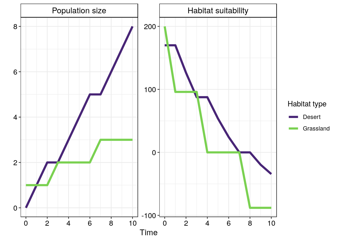
And we can do the same thing with the ideal-despotic model:

Use the Shiny App to help you explore these equations a little more and answer the questions that follow.

Download the habitat selection app here

Worksheet questions

Coding questions (17)

For this question you will need to produce the habitat selection model output for both models. The species you will be modelling is a clownfish which has the option of colonising either and undisturbed or bleached reef. Manipulate the code below to produce an output which resembles the figure beneath the code. You will need to identify four errors with the dataframe creation and then provide all the code to produce the figure itself. Submit your answers in a Word document format with comments or annotations explaining your correction to aid marking 15

# List of required packages for the script
list.of.packages <- c("dplyr", "tidyr", "ggplot2", "viridis")

# check if the required packages are already installed 
new.packages <- list.of.packages[!(list.of.packages %in% installed.packages()[,"Package"])]

# install missing ones
if(length(new.packages)) install.packages(new.packages, dependencies = TRUE) 

library(dplyr) # for data frame manipulation
library(tidyr) # for spreading and gathering  
library(ggplot2) # for plotting
library(viridis) # for cool colours

n = seq(from = 0, to = 15, by = 1) # the number of competitors to model

ifhs_df <- as.data.frame(n) # make this sequence of numbers into a dataframe

ifh1s_df <- ifhs_df %> # take this single column dataframe and pipe it into mutate
  mutate(Si = 300 - 2*n, 
         hab = "Undisturbed") %>% # mutate this dataframe by creating three new columns; Si, Ti (derrived from Si), and hab
    gather(key = "Suitability", value = "value") # gather the two new suitability columns in to a column called suitability and another one called value, ignore the n and hab columns
                      
ifh2s_df <- ifhs_df %>% 
  mutate(Si = 250 - 7*n, 
         hab = "Bleached") %>% 
    gather(key = "Suitability", value = "value") # do same as above but for the second habitat type

ifhs_df <- bind_rows(ifh1s_df, ifh2s_df)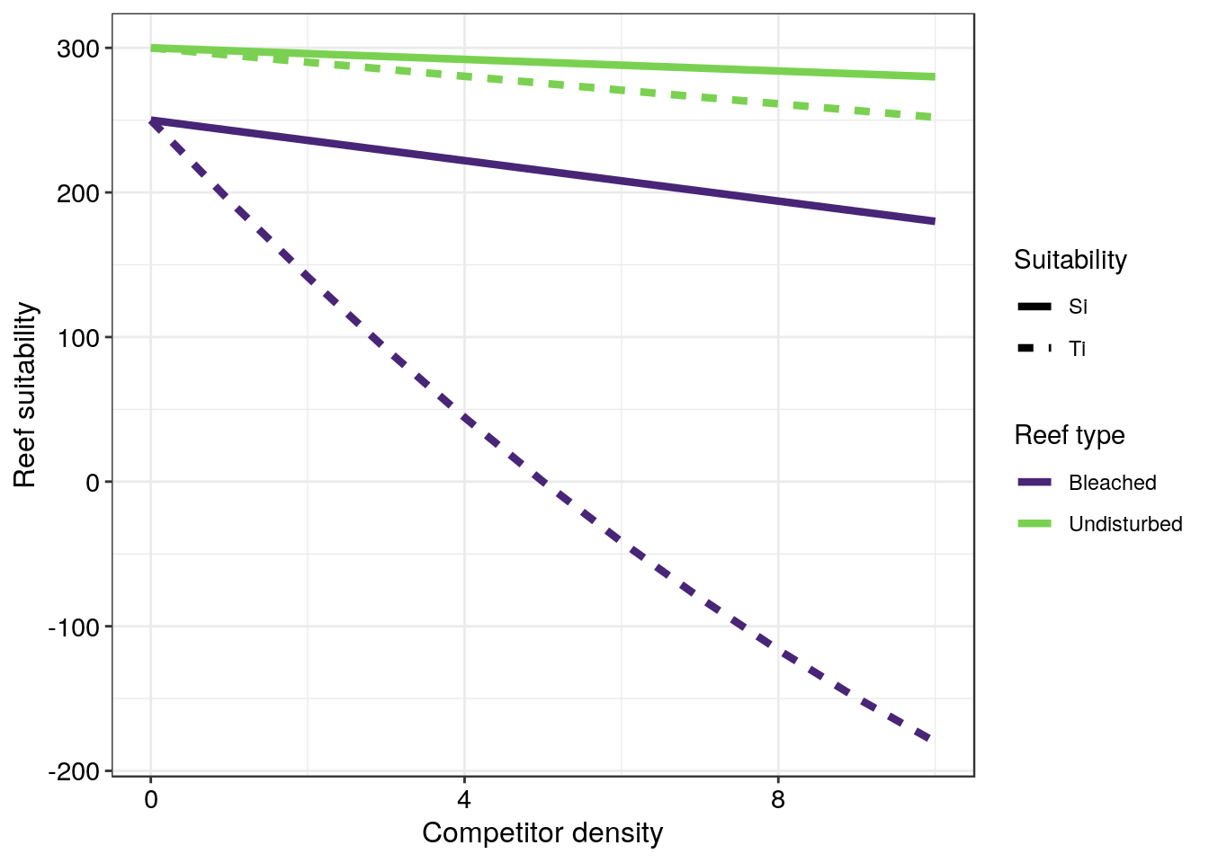

Application questions (35)

1. List and briefly explain three ecological factors that could be modelled by each of model parameters; \(S_i\), \(t_i\), and \(f_i\). For each explanation describe by means of ecological examples and reference to at least one scientific publication (i.e. 9 references are required for this question) the traits and characteristics that contribute importantly to the preference of one habitat type over another (3 x 3 x 3 = 27)

2. When a population has several similarly suitable habitats available to choose from the initial large population may split up into many smaller sub-populations. When these populations exchange individuals with one another the large population is referred to as a meta-population. Briefly describe and define the term “meta-population” (3) and discuss with reference to 3 different scientific articles (each addressing a different species) how conservationists and wildlife managers can employ meta-population theory to best manage at-risk animals populations (9) – (3 + 9 = 12)

3. Discuss the management implications and applications of the idea of habitat selection theory when managing wild populations in large, unfenced areas (11)